zkVM part III: from trace to polynomials
In part II, we covered the executor. The executor's main responsibility is to generate an execution trace of the program we want to prove. Before we can get to "proof of correct execution", we need a way to represent "correct execution"; the execution trace does just that.
You can think of the execution trace as a spreadsheet where each row corresponds to one step of the execution. Each column represents a part of the machine state (e.g., register values, memory contents) that is being recorded. Effectively, the execution trace is a comprehensive record of the program's entire computation.
Execution Trace as a Table
We have an execution trace which we can think of as a table. For illustrative purposes, let us take a look at a simplified table representing an execution trace:
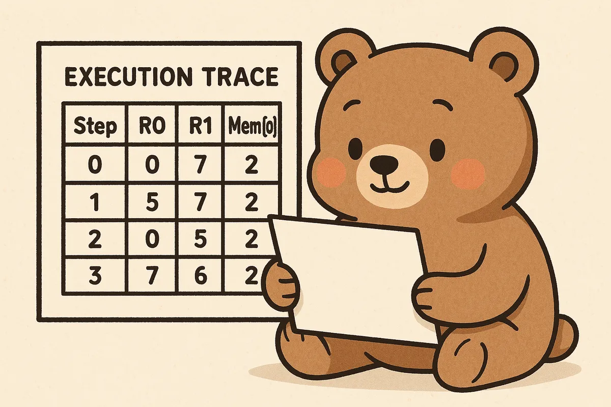
Step R0 R1 Mem[0]
0 0 0 2
1 5 0 2
2 7 5 2
3 7 6 2
where Step refers to each step in the execution; R0 and R1 are values stored in Registers 0 and 1 respectively; and Mem[0] refers to the first addressable word in memory.
The rows traverse over each "step" of the program, whereas the columns refer to specific values we're interested in. In the example above, for each step in the program, we are logging values in registers 0 and 1, and also the contents of the first address in memory.
To build on this, in a full execution trace, each row would match the complete state of the machine at each step or clock cycle in the computation. You may have heard the term cycles when benchmarking zkVM programs; a cycle is the smallest unit of compute in the zkVM and it is similar to the clock cycles in a physical CPU (typically measured in GHz these days). A rule of thumb is that a single cycle is required for most RISC-V operations (though some require two cycles).
1 weird trick to turn execution traces into polynomials — cryptographers love it!
Now that we have a cute small table, how can we start to think about it mathematically? (The reason why one might want to think about it mathematically will become obvious as we go on, patience is required!).
What would "thinking mathematically" here entail? How about plotting values on an x-y graph? If we read each column in the execution trace table as a sequence:
Column Sequence
Step [0, 1, 2, 3]
R0 [0, 5, 7, 7]
R1 [0, 0, 5, 6]
Mem[0] [2, 2, 2, 2]
To get four (x,y) points for each column, we treat the sequence of step points [0,1,2,3] as the x-values, and step through each sequence for the y-values. This way we can get four (x,y) points for each column in the execution trace:
- For the R0 column, the points are (0,0),(1,5),(2,7),(3,7)
- For R1, (0,0),(1,0),(2,5),(3,6)
- For Mem[0], (0,2),(1,2),(2,2),(3,2)
Using some magical polynomial interpolation (i.e. a way of finding a polynomial that goes through some specific points), we can find three polynomials PR0(x), PR1(x), PMEM0(x) which go through the points for each column.
Instead of getting bogged down in mathematical specifics here, let's keep it high level. The key idea here is that each column can be represented by a polynomial; one that passes through the four points we constructed above. We've gone from a table of data to just a few polynomials. This is called polynomial encoding.
What next?
We visualised an execution trace as a table, and we figured out how to map each column in the execution trace (that represents some interesting state in the computation like all the values of register X) to a polynomial.
A good question to ask here is "why did we go through all that hassle?". Part IV will cover how exactly these polynomial representations help us in our quest to generate a "proof of correct execution".